Originally published on Aylien's blog.
There has been a large resurgence of interest in generative models recently (see this blog post by OpenAI for example). These are models that can learn to create data that is similar to data that we give them. The intuition behind this is that if we can get a model to write high-quality news articles for example, then it must have also learned a lot about news articles in general. Or in other words, the model should also have a good internal representation of news articles. We can then hopefully use this representation to help us with other related tasks, such as classifying news articles by topic. Actually training models to create data like this is not easy, but in recent years a number of methods have started to work quite well. One such promising approach is using Generative Adversarial Networks (GANs). The prominent deep learning researcher and director of AI research at Facebook, Yann LeCun, recently cited GANs as being one of the most important new developments in deep learning:
"There are many interesting recent development in deep learning...The most important one, in my opinion, is adversarial training (also called GAN for Generative Adversarial Networks). This, and the variations that are now being proposed is the most interesting idea in the last 10 years in ML, in my opinion."— Yann LeCun
The rest of this post will describe the GAN formulation in a bit more detail, and provide a brief example (with code in TensorFlow) of using a GAN to solve a toy problem.
Discriminative vs. Generative models
Before looking at GANs, let’s briefly review the difference between generative and discriminative models:
- A discriminative model learns a function that maps the input data ($x$) to some desired output class label ($y$). In probabilistic terms, they directly learn the conditional distribution $P(y|x)$.
- A generative model tries to learn the joint probability of the input data and labels simultaneously, i.e. $P(x,y)$. This can be converted to $P(y|x)$ for classification via Bayes rule, but the generative ability could be used for something else as well, such as creating likely new $(x, y)$ samples.
Both types of models are useful, but generative models have one interesting advantage over discriminative models - they have the potential to understand and explain the underlying structure of the input data even when there are no labels. This is very desirable when working on data modelling problems in the real world, as unlabelled data is of course abundant, but getting labelled data is often expensive at best and impractical at worst.
Generative Adversarial Networks
GANs are an interesting idea that were first introduced in 2014 by a group of researchers at the University of Montreal lead by Ian Goodfellow (now at OpenAI). The main idea behind a GAN is to have two competing neural network models. One takes noise as input and generates samples (and so is called the generator). The other model (called the discriminator) receives samples from both the generator and the training data, and has to be able to distinguish between the two sources. These two networks play a continuous game, where the generator is learning to produce more and more realistic samples, and the discriminator is learning to get better and better at distinguishing generated data from real data. These two networks are trained simultaneously, and the hope is that the competition will drive the generated samples to be indistinguishable from real data.
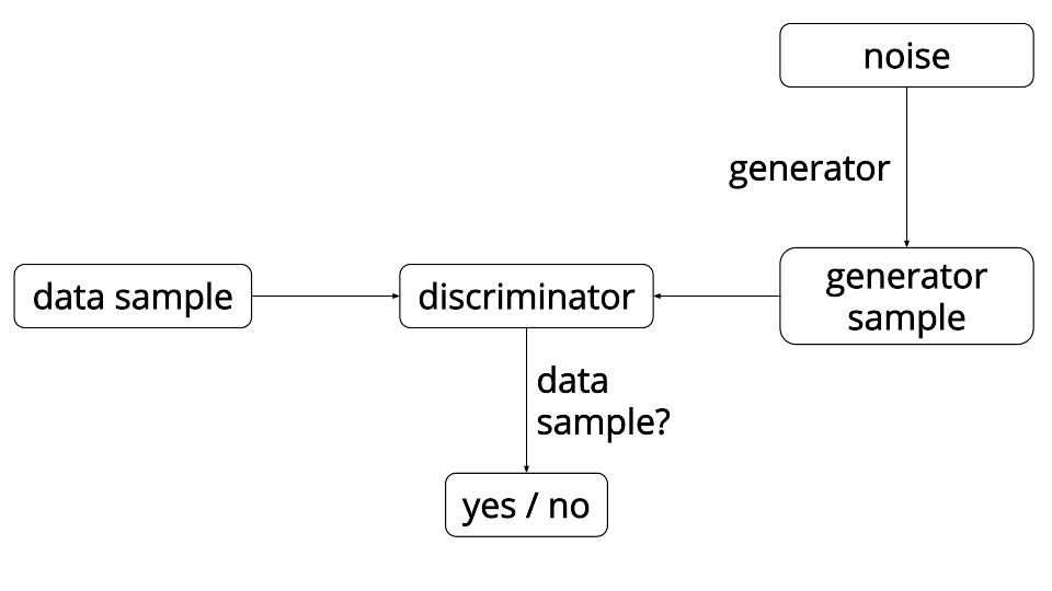
The analogy that is often used here is that the generator is like a forger trying to produce some counterfeit material, and the discriminator is like the police trying to detect the forged items. This setup may also seem somewhat reminiscent of reinforcement learning, where the generator is receiving a reward signal from the discriminator letting it know whether the generated data is accurate or not. The key difference with GANs however is that we can backpropagate gradient information from the discriminator back to the generator network, so the generator knows how to adapt its parameters in order to produce output data that can fool the discriminator.
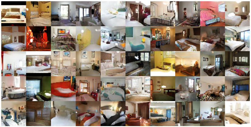
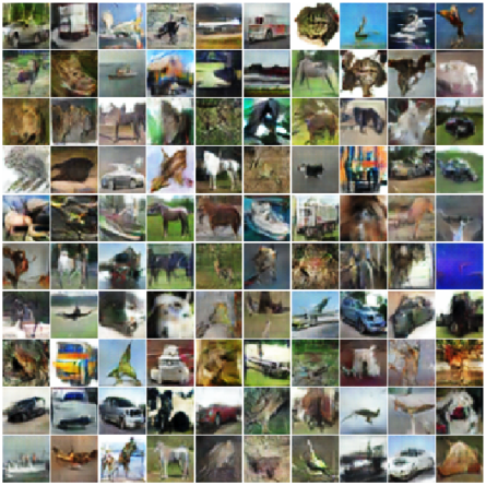
So far GANs have been primarily applied to modelling natural images. They are now producing excellent results in image generation tasks, generating images that are significantly sharper than those trained using other leading generative methods based on maximum likelihood training objectives. Here are some examples of images generated by GANs:
Approximating a 1D Gaussian distribution
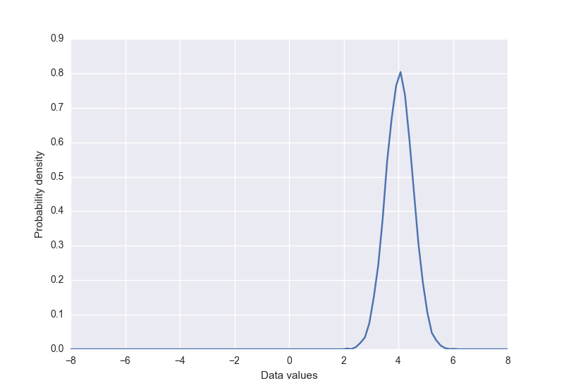
To get a better understanding of how this all works, we’ll use a GAN to solve a toy problem in TensorFlow - learning to approximate a 1-dimensional Gaussian distribution. This is based on a blog post with a similar goal by Eric Jang. The full source code for our demo is available on Github, here I will just focus on some of the more interesting parts of the code. First we create the "real" data distribution, a simple Gaussian with mean $4$ and standard deviation of $0.5$. It has a sample function that returns a given number of samples (sorted by value) from the distribution.
class DataDistribution:
    def __init__(self):
        self.mu = 4
        self.sigma = 0.5

def sample(self, N):
    samples = np.random.normal(self.mu, self.sigma, N)
    samples.sort()
    return samples
The data distribution that we will try to learn looks like this:
We also define the generator input noise distribution (with a similar sample function). Following Eric Jang’s example, I will also go with a stratified sampling approach for the generator input noise - the samples are first generated uniformly over a specified range, and then randomly perturbed.
class GeneratorDistribution:
    def __init__(self, range):
        self.range = range

def sample(self, N):
    return np.linspace(-self.range, self.range, N) + np.random.random(N) * 0.01
Our generator and discriminator networks are quite simple. The generator is a linear transformation passed through a nonlinearity (a softplus function), followed by another linear transformation.
def generator(input, hidden_size):
    h0 = tf.nn.softplus(linear(input, hidden_size, 'g0'))
    h1 = linear(h0, 1, 'g1')
    return h1
In this case I found that it was important to make sure that the discriminator is more powerful than the generator, as otherwise it did not have sufficient capacity to learn to be able to distinguish accurately between generated and real samples. So I made it a deeper neural network, with a larger number of dimensions. It uses tanh nonlinearities in all layers except the final one, which is a sigmoid (the output of which we can interpret as a probability).
def discriminator(input, hidden_size):
    h0 = tf.tanh(linear(input, hidden_size * 2, 'd0'))
    h1 = tf.tanh(linear(h0, hidden_size * 2, 'd1'))
    h2 = tf.tanh(linear(h1, hidden_size * 2, 'd2'))
    h3 = tf.sigmoid(linear(h2, 1, 'd3'))
    return h3
We can then connect these pieces together in a TensorFlow graph. We also define loss functions for each network, with the goal of the generator being simply to fool the discriminator.
with tf.variable_scope('G'):
    z = tf.placeholder(tf.float32, shape=(None, 1))
    G = generator(z, hidden_size)

with tf.variable_scope('D') as scope:
    x = tf.placeholder(tf.float32, shape=(None, 1))
    D1 = discriminator(x, hidden_size)
    scope.reuse_variables()
    D2 = discriminator(G, hidden_size)

loss_d = tf.reduce_mean(-tf.log(D1) - tf.log(1 - D2))
loss_g = tf.reduce_mean(-tf.log(D2))
We create optimizers for each network using the plain GradientDescentOptimizer in TensorFlow with exponential learning rate decay. It's important to note that finding good optimization parameters here did require some tuning.
def optimizer(loss, var_list):
    initial_learning_rate = 0.005
    decay = 0.95
    num_decay_steps = 150
    batch = tf.Variable(0)
    learning_rate = tf.train.exponential_decay(
        initial_learning_rate,
        batch,
        num_decay_steps,
        decay,
        staircase=True
    )

    optimizer = GradientDescentOptimizer(learning_rate).minimize(
        loss,
        global_step=batch,
        var_list=var_list
    )
    return optimizer

vars = tf.trainable_variables()
d_params = [v for v in vars if v.name.startswith('D/')]
g_params = [v for v in vars if v.name.startswith('G/')]

opt_d = optimizer(loss_d, d_params)
opt_g = optimizer(loss_g, g_params)
To train the model, we draw samples from the data distribution and the noise distribution, and alternate between optimizing the parameters of the discriminator and the generator.
with tf.Session() as session:
    tf.initialize_all_variables().run()

    for step in xrange(num_steps):
        # update discriminator
        x = data.sample(batch_size)
        z = gen.sample(batch_size)
        session.run([loss_d, opt_d], {
            x: np.reshape(x, (batch_size, 1)),
            z: np.reshape(z, (batch_size, 1))
        })

        # update generator
        z = gen.sample(batch_size)
        session.run([loss_g, opt_g], {
            z: np.reshape(z, (batch_size, 1))
        })
At the start of the training process, the generator was producing a very different distribution to the real data. It eventually learned to approximate it quite closely (somewhere around frame 750), before converging to a narrower distribution focused on the mean of the input distribution. After training, the two distributions look something like this:
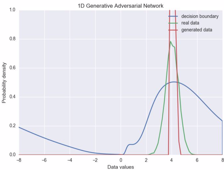
This makes sense intuitively. The discriminator is looking at individual samples from the real data and from our generator. If the generator just produces the mean value of the real data in this simple example, then it is going to be quite likely to fool the discriminator.
There are many possible solutions to this problem. In this case we could add some sort of early-stopping criterion, to pause training when some similarity threshold between the two distributions is reached. It is not entirely clear how to generalise this to bigger problems however, and even in the simple case, it may be hard to guarantee that our generator distribution will always reach a point where early stopping makes sense. A more appealing solution is to address the problem directly by giving the discriminator the ability to examine multiple examples at once.
Improving sample diversity
The problem of the generator collapsing to a parameter setting where it outputs a very narrow distribution of points is “one of the main failure modes” of GANs according to a recent paper by Tim Salimans and collaborators at OpenAI. Thankfully they also propose a solution: allow the discriminator to look at multiple samples at once, a technique that they call minibatch discrimination. In the paper, minibatch discrimination is defined to be any method where the discriminator is able to look at an entire batch of samples in order to decide whether they come from the generator or the real data. They also present a more specific algorithm which works by modelling the distance between a given sample and all other samples in the same batch. These distances are then combined with the original sample and passed through the discriminator, so it has the option to use the distance measures as well as the sample values during classification. The method can be loosely summarized as follows:
- Take the output of some intermediate layer of the discriminator.
- Multiply it by a 3D tensor to produce a matrix (of size num_kernels x kernel_dim in the code below).
- Compute the L1-distance between rows in this matrix across all samples in a batch, and then apply a negative exponential.
- The minibatch features for a sample are then the sum of these exponentiated distances.
- Concatenate the original input to the minibatch layer (the output of the previous discriminator layer) with the newly created minibatch features, and pass this as input to the next layer of the discriminator.
In TensorFlow that translates to something like:
def minibatch(input, num_kernels=5, kernel_dim=3):
    x = linear(input, num_kernels * kernel_dim)
    activation = tf.reshape(x, (-1, num_kernels, kernel_dim))
    diffs = tf.expand_dims(activation, 3) -
    tf.expand_dims(tf.transpose(activation, [1, 2, 0]), 0)
    abs_diffs = tf.reduce_sum(tf.abs(diffs), 2)
    minibatch_features = tf.reduce_sum(tf.exp(-abs_diffs), 2)
    return tf.concat(1, [input, minibatch_features])
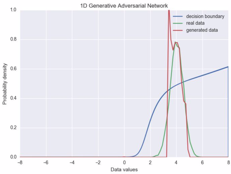
We implemented the proposed minibatch discrimination technique to see if it would help with the collapse of the generator output distribution in our toy example. The new behaviour of the generator network during training is shown below.
It’s clear in this case that adding minibatch discrimination causes the generator to maintain most of the width of the original data distribution (although it’s still not perfect). After convergence the distributions now look like this:
One final point on minibatch discrimination is that it makes the batch size even more important as a hyperparameter. In our toy example I had to keep batches quite small (less than around 16) for training to converge. Perhaps it would be sufficient to just limit the number of samples that contribute to each distance measure rather than use the full batch, but again this another parameter to tune.
Final thoughts
Generative Adversarial Networks are an interesting development, giving us a new way to do unsupervised learning. Most of the successful applications of GANs have been in the domain of computer vision, but here at Aylien we are researching ways to apply these techniques to natural language processing. If you’re working on the same idea and would like to compare notes then please get in touch. One big open problem in this area is how best to evaluate these sorts of models. In the image domain it is quite easy to at least look at the generated samples, although this is obviously not a satisfying solution. In the text domain this is even less useful (unless perhaps your goal is to generate prose). With generative models that are based on maximum likelihood training, we can usually produce some metric based on likelihood (or some lower bound to the likelihood) of unseen test data, but that is not applicable here. Some GAN papers have produced likelihood estimates based on kernel density estimates from generated samples, but this technique seems to break down in higher dimensional spaces. Another solution is to only evaluate on some downstream task (such as classification). If you have any other suggestions then we would love to hear from you.
More information
If you want to learn more about GANs I recommend starting with the following publications: