Deep learning can be seen as a continuation of research into artificial neural networks that has been going on for several decades. Although many people in the machine learning community decided that neural networks were a dead end and abandoned them in the 90s, it has turned out that with a few algorithmic changes, much bigger datasets and a lot more computational power, neural networks are once again state-of-the-art in some areas, and are once again mainstream news.

It is probably difficult for anyone working in tech to have missed the recent hype around the successes and future potential of deep learning, even if they're not directly working in the fields that have been largely affected by it such as speech recognition or computer vision (and more broadly machine learning and artificial intelligence). Deep nets can now help us with our much-loved past-time of looking at cats on the internet, they can play Atari games (when combined with reinforcement learning), and apparently some people are now so worried by the threat of our species engineering its own destruction at the hands of the machines that they are investing $1 billion in non-profit organisations just to try and keep things under control.

So, what better time to see if neural nets can help us make some music (or at least some musically-interesting sounds)?

This article describes a project that is still very much a work in progress, but I thought that some of this might be of interest to others. All of the code that is discussed here is available on Github.

Sound from recurrent neural networks

Audio generation seems like a natural application of recurrent neural networks, which are currently very popular (and effective) models for sequence-to-sequence learning. They have been used in speech recognition and speech synthesis, but I have not found many examples of RNNs being used to represent or create musical audio signals There are examples of using RNNs to generate higher-level musical structures such as chord sequences or entire pieces, but for this post at least, I am more interested in representing the low-level audio signals. The most recent related publication that I have found is this one from Saroff and Casey, although here they use autoencoders instead of RNNs.

If you have seen other work on this subject recently that I have missed then please let me know in the comments (or feel free to contact me directly).

(Edit: 2015-12-17) Thanks to Kyle Kastner for pointing out that Alex Graves has an interesting example of doing something similar with a vocoder on speech examples: see this video starting at 38 minutes.

(Edit: 2015-12-18) Thanks to Juan Hernandez for sending on this link to some more RNN-generated audio, this time from Aran Nayebi and Matt Vitelli at Stanford.

Modelling musical audio

A lot of the inspiration for this work comes from Alex Graves' work on handwriting synthesis, in which he shows that a recurrent neural network can be trained to represent and reproduce handwritten text. This is achieved by taking a sequence of online handwriting data - real-valued lists of (x, y) coordinates that represent the movement of the tip of a pen while writing - and feeding them into recurrent neural nets. The network learns to represent a probability distribution for the location of the next (x, y) location given the sequence that it has seen so far. For synthesis the network can be asked to generate a new (x, y) coordinate given an arbitrary starting point, then this data can be passed back into the network as input and the network asked to generate the next (x, y) coordinate, and so on. A logical extension of this work seems to be replace the pen-tip locations with other data sources, audio data for example.

When starting a new project, I generally find it useful to keep things as simple as possible. When it comes to musical audio, a logical first step is therefore to try modelling simple sound sources - in this case I chose some monophonic instrument samples (recordings of pitched instruments: clarinets, pianos, etc.). I have also spent some time working with this type of data in the past, and so was interested to see what sort of creative applications were presented by a change in representation.

I obviously don't want to have to build everything from scratch, so what deep learning libraries are already available? After a quick survey I decided to use Torch for this work (written in Lua). The level of abstraction of the neural net library seemed quite nice, and there are several great examples of Torch RNN models that served as a reference.

The model that I came up with looks like this (the various components are described briefly below):

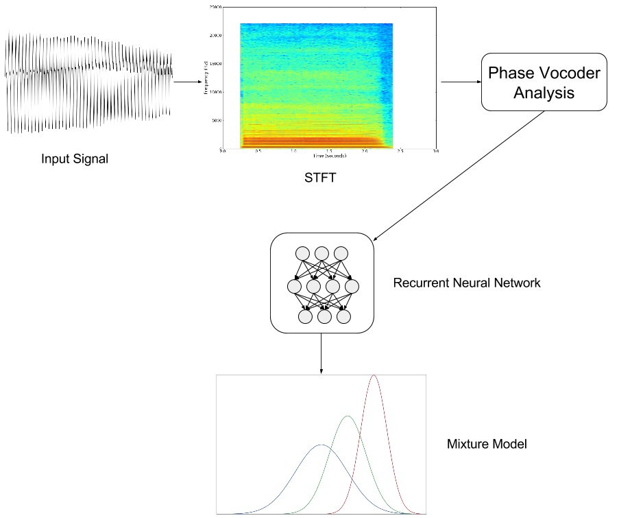
Input: the Phase Vocoder

There are several options for what sort of data could be used as input for the RNN - raw audio samples, short-time Fourier transform (STFT) coefficients, sinusoidal models, etc. I decided to use the Phase Vocoder. Training a model from end-to-end starting with the raw audio is interesting, but I suspected that it would potentially take quite a large model to come up with anything that sounds reasonable (therefore taking a long time to train), and may also be more problematic to debug. I wanted to be able to get something working quickly and so passed on this idea for now, but it is worth exploring at a later date. I'm quite fond of sinusoidal models, but they bring a level of complexity that I was hoping to avoid here. The Phase Vocoder seemed like a reasonable compromise between the two.

I won't go into much detail explaining how the Phase Vocoder works, but the basic idea is:

• Take a STFT of the input signal.
• Extract the magnitude and phase components.
• The STFT magnitudes only refer to the frequency of the bin centre frequency. The bin bandwidth can be quite large (depending on the FFT size), but you can get a more accurate estimate of the sinusoidal frequency that is present in each bin by looking at the rate of change of phase between the same bin number in successive frames. Use this to produce a set of (magnitude, frequency) tuples for each frame.
• The magnitudes and frequencies can now be manipulated independently, in this case by passing them through a RNN.
• In resynthesis the procedure can be inverted - the original signal is reconstructed by taking magnitudes and frequencies, computing the inverse STFT, and summing overlapping windowed frames.

The code for my Torch Phase Vocoder implementation is in the Github repository, so take a look if you're interested in the details. It is based on Victor Lazzarini's implementation in The Audio Programming Book, so if you want to know more about how this works then that is a good place to start (I also wrote the chapter on Sinusoidal Modelling on the DVD that comes with the book). I have made one small addition to the use Phase Vocoder implementation: making it possible to limit the number of spectral components that are used. This effectively throws away the data from every bin with an index greater than the specified limit and so acts as a low-pass filter. This is primarily to be able to reduce the dimensionality of the input data in a way that makes some sense musically, as the highest frequencies will in general be less perceptually significant. The code itself could probably be improved significantly by vectorising the operations, but as the Phase Vocoder is only run before RNN training and after sample generation this doesn't really influence the overall training time which is dominated by learning the RNN weights.

Long Short-Term Memory network

The next layer of the model is a recurrent neural network, which in the most simple formulation can be viewed as a traditional feedforward network where the output of some layers feed back into their input. This allows the output of the network to depend on previous input values, as well as on the current input. Unlike traditional neural networks (and the Convolutional Neural Networks that are now extremely popular for image recognition), RNNs therefore do not have a fixed-size input vector, and so can operate over sequences of input values. These inputs are then combined with an internal state in a fixed (but learnable) way, producing a new output vector.

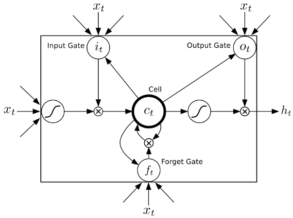
Technically I'm actually using a particular type of RNN structure called a Long Short-Term Memory (LSTM). They are more complicated structures that make use of several gates to control the flow of data both in and out of the central LSTM cell (see the diagram below). These gates are basically switches that take values between 0 and 1, but they are smooth (and differentiable). Notice that the same input vector x_t is used as the input to the various gates. LSTMs have been found to be better at finding and exploiting long range dependencies in data than traditional RNNs. For more on LSTMs see Hochreiter and Schmidhuber or this blog post.

Mixture density outputs

What should the LSTM actually try to learn? One possibility would be to minimise the mean squared error between the network outputs at time t and the input sequence at time t + 1. However as Bishop describes, the least squares technique can be derived from maximum likelihood if you assume (uni-modal) Gaussian distributed data. Or in other words for a given input vector, the network will converge towards a single average output vector.

As simply finding the average output for a given sequence often does not seem particularly useful when working with real-valued data, a typical alternative is to instead learn to replace the single Gaussian with a mixture of Gaussians. A feedforward neural network that feeds a Gaussian mixture model is called a Mixture Density Network. The mixture model may also be fed by RNNs (see Graves), where the network learns to compute the weights, means and variances that parameterise the Gaussian mixture model. Technically with enough hidden layers and mixture components these networks can approximate (as closely as desired) any probability density, but as always there will be a trade off between how powerful the model is and how long it takes to train.

I implemented a mixture density output layer as a Torch criterion. For anyone interested in the math behind the implementation, Schuster's "On supervised learning from sequential data with applications for speech recognition" gives the gradient equations for the multivariate Gaussian mixture. I decided to use a diagonal covariance matrix instead of the more simple single variance per mixture component formulation that is also given in the Schuster paper. This means that there is 1 variance value per input dimension per mixture component, which I expect to be useful as the magnitude and frequency values in each spectral bin may evolve quite differently. The model cannot model the correlations that may exist between input components however, but in practise I am hoping that this is not too much of a problem.

Sine waves

To make sure that the model was working as expected, I first decided to test it on what should be the most basic of input sources - a single sine wave (in this case at 440 Hz):

A model was trained on this data with the following audio parameters:

• FFT size: 512
• Hop size: 128
• Number of spectral components: 10

It used the following RNN parameters:

• Number of LSTM layers: 1
• Number of LSTM units per layer: 100
• LSTM sequence length: 10
• Number of mixture density components: 1

The model was trained using stochastic gradient descent (with AdaGrad).

After training for several minutes on my laptop's CPU, that resulted in something that sounds like this when sampled:

Not amazingly close, but not hugely far away either (there is a vague sense of pitch at least). Time to take a closer look at the data to see what is going on. The input (after Phase Vocoder analysis) consists of a set of magnitude and frequency pairs. There is some noise due to sampled nature of the FFT (and the analysis windowing), but a typical frame of audio data produced results that look like this:

Component	Magnitude	Frequency
0	0.0000	0.0000
1	0.0288	73.1652
2	0.0626	90.0327
3	0.2284	94.5254
4	6.7281	439.9791
5	15.8478	440.0076
6	9.3078	439.9927
7	0.3617	440.1625
8	0.0839	785.0665
9	0.0329	785.5969

There is a clear peak at around 440 Hz, but the energy is spread over several frequency bins. There is not much frame-to-frame variance in these numbers, as you would expect with a steady sine wave. The model in comparison was producing a typical frame that looked like this:

Component	Magnitude	Frequency
0	0.0225	27.8832
1	0.3056	68.0510
2	-0.1558	-2.1814
3	0.0021	79.9063
4	6.6045	445.7344
5	15.9591	439.5001
6	9.3758	436.5928
7	0.4158	381.9936
8	0.0173	780.6247
9	-0.0879	777.9229

There are some values that are quite far from ideal (the frequencies in bins 2 and 7), but most values seem reasonably close to the originals. When looking at multiple frames though the problem became clear, there is too much variance in the synthesised frames. Reducing the variance by 10^-5 produces something that sounds like this:

Much cleaner. The variance seemed to be decreasing between successive training batches so it seems that the model is correctly learning as expected, although quite slowly considering how simple the data is. You may also have noted that this already suggests one possible sound transformation - changing the variance of the model over time.

Changes over time

So, the model can learn to represent real-valued sequences of Phase Vocoder output, but musically it will be much more interesting and powerful if the model can learn to represent the way in which these values change over time, rather than the sequence of absolute values themselves. If we model how much the magnitude and frequency is changing in each spectral band, then many musical transformations are possible - changing the rate at which these values vary (time-stretching), mapping the changes from one sound source onto another (some sort of spectral cross-synthesis), etc.

It is a small code change to pass the differences between corresponding bins in successive frames to the RNN instead of the absolute values. How does the output of the model change? We now get something that sounds like this:

It now has the tendency for the centre frequency to drift slightly over time, but still sounds reasonably close to the original.

Clarinet

Single sine waves are easy to deal with, how about something a bit more complicated? I modelled the following clarinet sound:

with these parameters:

• FFT size: 512
• Hop size: 128
• Number of spectral components: 20
• Number of LSTM layers: 2
• Number of LSTM units per layer: 100
• LSTM sequence length: 20
• Number of mixture density components: 3

After spinning up and instance and leaving this to train for several hours (still only on CPUs), the result was this:

Here the drift in the frequencies of the sinusoidal components is much more evident. This reminded me of a similar problem that exists in data compression when delta coding schemes are used, and one solution there is to add one uncompressed frame at regular intervals (which basically acts as a reset). If we do something similar here, adding 1 frame selected randomly from around the middle of a source audio file a few times per second, we get something more like this:

If we now reduce the model variance during sampling:

Much improved, and again suggesting room for creative potential in changing what sound source is used to "reset" the frequency deltas. It would obviously be better if this was not required, although it's important to emphasise that this is just a toy model by current deep learning standards (around 160000 parameters) and was not trained for very long.

Piano

This is currently far from being a panacea for modelling all musical audio sounds however. Even taking a sound that is still relatively simple, this piano note:

modelled with the following parameters:

• FFT size: 2048
• Hop size: 512
• Number of spectral components: 20
• Number of LSTM layers: 2
• Number of LSTM units per layer: 150
• LSTM sequence length: 20
• Number of mixture density components: 5

produced the following after several hours of training:

I haven't yet taken the time to figure out what is going on here, but clearly this is far removed from the original sound.

Closing thoughts

It was fun to play around with recurrent neural networks for musical audio, but there is still quite a long way to go before this approach will replace existing techniques for sound transformation. As I mentioned above, these are really only toy models. It would be interesting to see how these perform if scaled up, given considerably more input data, and allowed to train for a much longer time.

The code is all on Github for those who are interested in playing with this, have fun :)